2. Vanilla GAN 구현

Posted May 2, 2024

By JUNHEE LEE

14 min read

Vanilla Generative Adversarial Networks(GAN)

Imports

  
import time
import numpy as np
import torch
import torch.nn.functional as F
from torchvision import datasets
from torchvision import trnasforms
import torch.nn as nn
from troch.utils.data import DataLoader

if torch.cuda.is_available():
	torch.backends.cudnn.deterministic = True

Settings and Dataset

  
# Device
device = torch.device("cuda:3" if torch.cuda.is_available() else "cpu")

# Hyperparameters
random_seed = 123
generator_learning_rate = 0.001
discriminator_learning_rate = 0.001
num_epochs = 100
batch_size = 128

LATENT_DIM = 100 # 잠재 공간(latent space)의 차원을 정의
# GAN에서 Generator는 잠재 공간에서 무작위로 샘플링한 벡터를 입력받아 실제 데이터와 유사한 데이터를 생성 
# 여기서 LATENT_DIM은 잠재 벡터의 차원 수를 의미하며, 이 경우 100차원의 벡터를 사용한다는 것을 의미 
# 100차원 벡터는 100개의 요소를 가진 리스트 또는 배열 
# [1, 2, 3]은 3차원 벡터 
# [0.1, -0.2, 0.3, ..., 0.5] 100차원 벡터 

IMG_SHAPE = (1, 28, 28)
IMG_SIZE = 1
for x in IMG_SHAPE: # (1, 28, 28)이라면, IMG_SIZE는 784
	IMG_SIZE *= x


# Note transforms.ToTensor() scales input images
# to 0-1 range
train_dataset = datasets.MNIST(root = 'data',
							   train = True,
							   transform = transforms.ToTensor(),
							   download=True)
							   
test_dataset = datasets.MNIST(root = 'data',
							  train = False,
							  transform = transforms.ToTensor())


train_loader = DataLoader(dataset = train_dataset,
						  batch_size = batch_size, 
						  shuffle = True)
						  
test_loader = DataLoader(dataset = test_dataset, 
						 batch_size = batch_size,
						 shuffle = False)

for images, labels in train_loader: 
	print("Image batch dimensions:", images.shape)
	print("Image label dimensions:", labels.shape)
	break

"""
Image batch dimensions: torch.Size([128, 1, 28, 28])
Image label dimensions: torch.Size([128])
"""

Model

  
class GAN(torch.nn.Module):
	def __init__(self):
		super(GAN, self).__init__()

		self.generator = nn.Sequential(
			nn.Linear(LATENT_DIM, 128), # 100개 랜덤 노이즈 입력
			nn.LeakyReLU(inplace = True),
			"""
			연산을 수행함으로써 생성되는 중간 결괄르 새로운 메모리 공간에 저장하는 대신, 입력 텐서를 직접 수정해 결과를 저장.
			
			주의!
			inplace 연산은 원본 데이터를 변경하기 때문에, 해당 데이터가 연산 과정에서 다시 사용되야 할 경우 문제가 발생 할 수 있다.
			연산의 중간 결과가 나중에 그래디언트 계산에 필요할 경우 inplace = True를 사용하면 역전파 단계에서 오류가 발생할 수 있다
			ex) Concatenate, Residual Connections
			"""
			nn.Dropout(p=0.5),
			nn.Linear(128, IMG_SIZE), # 이미지 사이즈로 출력 
			nn.Tanh()
		)

		self.discriminator = nn.Sequential(
			nn.Linear(IMG_SIZE, 128), # 이미지 입력
			nn.LeakyReLU(inplace = True),
			nn.Dropout(p=0.5),
			nn.Linear(128, 1), # 출력은 확률
			nn.Sigmoid()
		)

	def generator_forward(self, z):
		img = self.generator(z)
		return img

	def discriminator_forward(self, img):
		pred = self.discriminator(img)
		return pred.view(-1)

  
torch.manual_seed(random_seed)

model = GAN()
model = model.to(device)

optim_gener = torch.optim.Adam(model.generator.parameters(), lr = generator_learning_rate)
optim_discr = torch.optim.Adam(model.discriminator.parameters(), lr = discriminator_learning_rate)

model 

"""
GAN(
  (generator): Sequential(
    (0): Linear(in_features=200, out_features=128, bias=True)
    (1): LeakyReLU(negative_slope=0.01, inplace=True)
    (2): Dropout(p=0.5, inplace=False)
    (3): Linear(in_features=128, out_features=784, bias=True)
    (4): Tanh()
  )
  (discriminator): Sequential(
    (0): Linear(in_features=784, out_features=128, bias=True)
    (1): LeakyReLU(negative_slope=0.01, inplace=True)
    (2): Dropout(p=0.5, inplace=False)
    (3): Linear(in_features=128, out_features=1, bias=True)
    (4): Sigmoid()
  )
)
"""

왜 `model.train()`과 `model.eval()`을 사용해야 하는가?

model.train(): 이 메서드를 호출하면 모델을 학습 모드로 설정된다. 학습 모드에서는 Dropout 층이 활성화되어 뉴런을 임의로 끄고, BatchNorm 층은 현재 배치의 데이터를 기반으로 평균과 분산을 계산하여 적용한다. 이는 모델이 학습할 때 올바르게 동작하도록 한다.
model.eval(): 이 메서드를 호출하면 모델을 평가(추론) 모드로 설정한다. 평가 모드에서는 Dropout 층이 비활성화되어 모든 뉴런이 활성 상태를 유지하고, BatchNorm 층은 학습 중에 계산된 이동 평균(moving average)과 이동 분산(moving variance)을 사용한다. 이는 모델이 추론할 때 일관된 성능을 보이도록 한다.
PyTorch 모델은 기본적으로 학습 모드(train)로 초기화된다. 그러나 명시적으로 모드를 전환하는 것이 좋은 이유는 학습과 평가 시에 모델의 동작을 명확하게 제어하기 위함이다.

Training

  
# 시작 시간 기록
start_time = time.time()

# 판별자와 생성자의 손실을 기록할 리스트를 초기화
discr_costs = []
gener_costs = []

# 지정된 epoch 수만큼 학습을 반복
for epoch in range(num_epochs):
	# 모델을 학습 모드로 설정
	model.train()
	# 데이터 로더를 통해 학습 데이터의 배치를 순회
	for batch_idx, (features, targets) in enumerate(train_loader):
		features = (features - 0.5) * 2
		# 입력 이미지 데이터를 [-1, 1] 범위로 정규화
		"""
		입력 데이터의 픽셀 값을 정규화하는 과정.
		MNIST 데이터셋의 각 이미지는 0에서 255 사이의 픽셀값을 가지고, 
		transform=transforms.ToTensor() 를 통해 이를 0에서 1 사이의 값으로 변환
		이 변환은 모델 학습에 있어 입력 데이터의 스케일을 일정하게 맞추어 주기 위한 전처리 단계중 하나.
		그러나, 더 나아가 데이터를 [-1, 1]범위로 다시 정규화. 이는 데이터의 중심을 0으로 옮기고, 범위를 -1부터 1까지로 확장하여 
		모델이 데이터를 더 잘 학습할 수 있도록 돕는다.

		1. 중심화(Centering): 데이터의 평균을 0으로 만들어, 모델이 패턴을 더 쉽게 인식할 수 있도록 한다. 중심이 0이 되면, 가중치 업데이터가 더 안정적이고 효율적으로 이뤄질 수 있다. 

		2. 스케일 조정(Scaling): 데이터의 범위를 [-1, 1]로 조정하여, 모든 특성들이 비슷한 스케일을 가지게 함으로써, 
		학습 과정에서의 가중치 업데이트가 더 균등하게 이뤄지도록 한다.
		"""
		# 이미지 데이터를 적절한 크기로 변형하고, 계산에 사용될 장치로 옮김
		features = features.view(-1, IMG_SIZE).to(device) # == tf.reshape(-1, 784) == (배치(여기서는 128, 784)

		# 타겟 데이터(여기서는 사용되지 않음)를 계산에 사용할 장치로 옮김
		targets = targets.to(device)

		# 진짜 데이터에 대한 레이블을 나타내는 텐서를 생성 
		# targets.size() = torch.Size([128]),  targets.size(0) = 128

		valid = torch.ones(targets.size(0)).float().to(device) 
		# 가짜 데이터에 대한 레이블을 나타내는 텐서를 생성 
		fake = torch.zeros(targets.size(0)).float().to(device)


		### FORWARD AND BACK PROPAGATION 
		# -------------------------- 

		# 생성자 학습
		# --------------------------
		# 잠재 공간에서 무작위 노이즈를 생성 
		z = torch.zeros((targets.size(0), LATENT_DIM)).uniform_(-1.0, 1.0).to(device)

		# 생성자를 사용해 노이즈로부터 이미지를 생성 
		generated_features = model.generator_forward(z)

		# 생성된 이미지를 판별자에 입력하여 진짜 이미지로 분류되게 하는 손실을 계산
		discr_pred = model.discriminator_forward(generated_features

		gener_loss = F.binary_cross_entropy(discr_pred, valid)
		"""
		진짜 데이터에 해당하는 레이블을 텐서에 생성. GAN에서 Discriminator가 진짜 데이터와 가짜 데이터를 구분하도록 학습되는데, 
		진짜 데이터에 대한 레이블은 1로, 가짜 데이터에 대한 레이블은 0으로 설정.

		gener_loss = F.binary_cross_entropy(discr_pred, valid) 이는 생성자의 손실을 계산하는 부분으로 생성자의 목표는 판별자를 속여 
		가짜 데이터를 진짜 데이터로 분류하게 만드는것. 여기서 discr_pred 는 판별자가 생성된 이미지에 대해 출력한 예측값.
		이 예측값은 생성된 이미지가 진짜일 확률을 나타낸다.

		F.binary_cross_entropy 는 이진 교차 엔트로피(BCEE) 손실 함수로, 두 확률 분포간의 차이를 측정.
		이 경우, 하나의 분포는 Discriminator의 예측값, 다른 하나는 진짜 데이터에 해당하는 레이블(valid).
		생성자는 판별자가 생성된 이미지를 진짜로 잘못 분류하게 만들고자 하므로, valid 텐서는 모두 1로 설정. 이는 Discriminator가 생성된 
		이미지를 진짜로 판별할 확률을 최대화하려는 생성자의 목표를 반영
		"""

		# 생성자의 그래디언트를 초기화하고, 역전파를 통해 그래디언트를 계산한 후, 최적화 스텝을 수행 
		optim_gener.zero_grad()
		gener_loss.backward()
		optim_gener.step()



		# -------------------------- 
		# 판별자 학습
		# --------------------------

		# 진짜 이미지를 판별자에 입력해 손실을 계산 
		discr_pred_real = model.discriminator_forward(features.view(-1, IMG_SIZE))
		real_loss = F.binary_cross_entropy(discr_pred_real, valid)

		# 생성된 가짜 이미지를 판별자에 입력하여 손실을 계산 
		discr_pred_fake = model.discriminator_forward(generated_features.detach())
		fake_loss = F.binary_cross_entropy(discr_pred_fake, fake)

		# 진짜 이미지와 가짜 이미지에 대한 손실을 평균내어 최종 판별자 손실을 계산 
		discr_loss = 0.5 * (real_loss + fake_loss) 

		# 판별자의 그래디언트를 초기화하고, 역전파을 통해 그래디언트를 계산한 후, 최적화 스텝을 수행
		optim_discr.zero_grad()
		discr_loss.backward()
		optim_discr.step()

		# 판별자와 생성자의 손실을 기록 
		discr_costs.append(discr_loss.item())
		gener_costs.append(gener_loss.item())


		### Logging
		# 지정된 배치마다 학습 진행 상황을 출력(매 100번째 배치마다 진행 상황을 출력. 배치 사이즈와 무관)
		# ex) batch_idx 가 0이면 배치 사이즈의 갯수 데이터가 처리중인 상태
		if not batch_idx % 100:
			print ('Epoch: %03d/%03d | Batch %03d/%03d | Gen/Dis Loss: %.4f/%.4f'
					%(epoch+1, num_epochs, batch_idx,
			len(train_loader), gener_loss, discr_loss))
	
	# 에폭당 경과 시간 출력
	print('Time elapsed: %.2f min' % ((time.time() - start_time)/60))

# 전체 학습 시간 출력
print('Total Training Time: %.2f min' % ((time.time() - start_time)/60))	


"""
Time elapsed: 11.18 min
Epoch: 100/100 | Batch 000/469 | Gen/Dis Loss: 0.8612/0.6245 
Epoch: 100/100 | Batch 100/469 | Gen/Dis Loss: 0.8867/0.6514 
Epoch: 100/100 | Batch 200/469 | Gen/Dis Loss: 0.8036/0.6459 
Epoch: 100/100 | Batch 300/469 | Gen/Dis Loss: 0.8861/0.6495 
Epoch: 100/100 | Batch 400/469 | Gen/Dis Loss: 0.8458/0.6326 
Time elapsed: 11.29 min 
Total Training Time: 11.29 min
"""

Evaluation

  
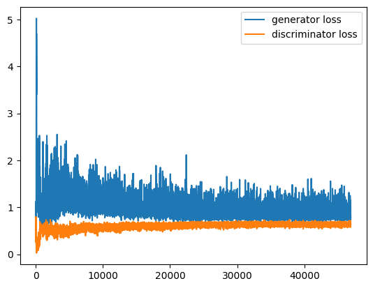
import matplotlib.pyplot as plt

plt.plot(range(len(gener_costs)), gener_costs, label='generator loss')
plt.plot(range(len(discr_costs)), discr_costs, label='discriminator loss')
plt.legend()
plt.show()

  
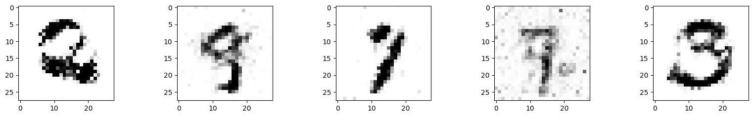
model.eval()

# Make new images
z = torch.zeros((5, LATENT_DIM)).uniform_(-1.0, 1.0).to(device)
generated_features = model.generator_forward(z)
imgs = generated_features.view(-1, 28, 28)

fig, axes = plt.subplots(nrows=1, ncols=5, figsize=(20, 2.5))

for i, ax in enumerate(axes):
	axes[i].imshow(imgs[i].to(torch.device('cpu')).detach(), cmap='binary')

논문구현, GenerativeModels

GANs Vanilla GAN

This post is licensed under CC BY 4.0 by the author.

Vanilla Generative Adversarial Networks(GAN)

Imports

Settings and Dataset

Model

왜 model.train()과 model.eval()을 사용해야 하는가?

Training

Evaluation

Trending Tags

왜 `model.train()`과 `model.eval()`을 사용해야 하는가?