7. U-Net (Gray to Color)
데이터 소개
- portrait 데이터로 유명한 PFCN dataset 사용
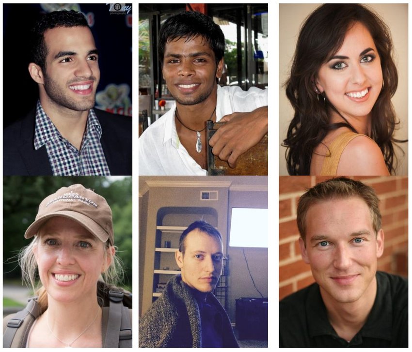
이미지는 다음과 같은 것을 보여준다.
- 800 x 600의 사람 portrait 이미지
- 사람 영역에 대한 흑백 portrait 이미지
- pfcn_original
- 원본 800 x 600 이미지들
- pfcn_small
- colab용 100 x 75 이미지들
최종 목표
- 작게 줄인 PFCN 데이터를 이용해 사람 영역 추출
- 코앱에 구글 drive 연동
- 큰 사진을 작게 줄이기
- 이미지에 대한 오토인코더식 접근 방법
- 흑백 사진을 칼라 사진으로 만드는 모델 이해
전처리
1
2
3
4
5
6
7
"""
데이터 로드
"""
datasets = np.load('datasets/pfcn_small.npz')
print(list(datasets.keys()))

train_images, test_images = datasets['train_images'], datasets['test_images']
1
2
3
4
5
6
7
8
9
10
11
"""
흑백 이미지 생성
"""
from skimage import color

train_gray_images = np.array([color.rgb2gray(img).reshape(100, 75, 1) for img in train_images])
test_gray_images = np.array([color.rgb2gray(img).reshape(100, 75, 1) for img in test_images])

# (N, 100, 75, 1)
plt.imshow(train_gray_images[:5].transpose(1, 0, 2, 3).reshape(100, -1, 1), cmap = 'gray')
plt.show()
흑백 이미지를 칼라로 변환하는 모델링 U-Net
1
2
3
4
5
6
7
8
9
10
11
12
13
14
15
16
17
18
19
20
21
22
23
24
25
26
27
28
29
30
31
32
33
34
35
36
37
38
39
40
41
42
43
44
45
46
47
48
49
50
51
52
53
54
55
56
57
58
59
60
61
62
63
64
65
66
67
68
69
70
71
72
73
74
75
76
77
78
79
80
81
from keras.layers import Dense, Input, MaxPool2D, Conv2D, Conv2DTranspose, Flatten, Reshape, Activation
from keras.layers import BatchNormalization, Dropout, Activation, concatenate
from keras.models import Model


def conv2d_block(x, channel):
	x = Conv2D(filters=channel, kernel_size=3, padding='same')(x)
	x = BatchNormalization()(x)
	x = Activation('relu')(x)

	x = Conv2D(filters=channel, kernel_size=3, padding='same')(x)
	x = BatchNormalization()(x)
	x = Activation('relu')(x)
return x


def unet_color():
	inputs = Input(shape=(100, 75, 1))
	c1 = conv2d_block(inputs, 16)
	p1 = MaxPool2D(pool_size=(2))(c1)
	p1 = Dropout(0.1)(p1)

	c2 = conv2d_block(p1, 32)
	p2 = MaxPool2D(pool_size=(2))(c2)
	p2 = Dropout(0.1)(p2)

	c3 = conv2d_block(p2, 64)
	p3 = MaxPool2D(pool_size=(2))(c3)
	p3 = Dropout(0.1)(p3)

	c4 = conv2d_block(p3, 128)
	p4 = MaxPool2D(pool_size=(2))(c4)
	p4 = Dropout(0.1)(p4)

	c5 = conv2d_block(p4, 256)

	u6 = Conv2DTranspose(128, kernel_size=2, strides=2, padding='valid', output_padding=(0, 1))(c5)
	u6 = concatenate([u6, c4])
	u6 = Dropout(0.1)(u6)
	c6 = conv2d_block(u6, 128)

	u7 = Conv2DTranspose(64, kernel_size=2, strides=2, padding='valid', output_padding=(1, 0))(c6)
	u7 = concatenate([u7, c3])
	u7 = Dropout(0.1)(u7)
	c7 = conv2d_block(u7, 64)

	u8 = Conv2DTranspose(32, kernel_size=2, strides=2, padding='valid', output_padding=(0, 1))(c7)
	u8 = concatenate([u8, c2])
	u8 = Dropout(0.1)(u8)
	c8 = conv2d_block(u8, 32)

	u9 = Conv2DTranspose(16, kernel_size=2, strides=2, padding='valid', output_padding=(0, 1))(c8)
	u9 = concatenate([u9, c1])
	u9 = Dropout(0.1)(u9)
	c9 = conv2d_block(u9, 16)

	outputs = Conv2D(filters = 3, kernel_size = 1, activation = 'sigmoid')(c9)

	model = Model(inputs, outputs)

return model

model = unet_color()

model.compile(loss = 'mae', optimizer = 'adam', metrics=['accuracy'])

hist = model.fit(
	train_gray_images,
	train_images,
	validation_data=(
		test_gray_images,
		test_images
	),
	epochs= 50,
	verbose=1
)


res = model.predict(test_gray_images[1:2])
plt.imshow(np.concatenate([res[0], test_images[1]], axis = 1))
plt.show()
결과 확인
1
2
3
4
5
6
"""
모델 사진 위 5장 실제 사진 아래 5장
"""
res_five = model.predict(test_gray_images[:5])
plt.imshow(np.concatenate([res_five, test_images[:5]], axis = 1).transpose(1, 0, 2, 3).reshape(200, -1, 3))
plt.imshow
_1.png)
Lab 칼라 모델링
Lab color:
사진이나 이미지 처리에서 사용되는 색 공간 모델로 Lab 색 공간은 인간의 시각에 가깝게 설계되었으며, 다른 색 공간들과 달리 장치에 독립적. 이것은 Lab 색 공간이 특정 프린터, 모니터 또는 카메라에 의존하지 않는다는 것을 의미.
Lab 색 공간 세 가지 구성 요소
- L (Luminance): 밝기를 나타내며 L값은 0에서 100 사이에서 변화하며, 0은 완전한 검정, 100은 완전한 백색을 나타낸다.
- a (from Green to Magenta): 색의 녹색에서 자홍색까지의 색상 구성 요소이다. 이 축에서 음수 값은 녹색을, 양수 값은 자홍색을 나타낸다.
- b (from Blue to Yellow): 색의 청색에서 황색까지의 색상 구성 요소이다. 이 축에서 음수 값은 청색을, 양수 값은 황색을 나타낸다.
Lab 색 공간의 주요 이점 중 하나는 인간의 색상 인식과 유사한 방식으로 색상을 나타낸다는 것이다. 이는 색상의 작은 차이도 잘 구분할 수 있게 해준다. 또한, 다양한 장치에서 일관된 색상을 재현하는 데 유용하다.
1
2
3
4
5
6
"""
RGB to lab color
"""

train_lab_images = np.array([color.rgb2lab(img) for img in train_images])
test_lab_images = np.array([color.rgb2lab(img) for img in test_images])
1
2
3
4
5
6
7
8
9
10
11
12
13
14
15
16
17
18
19
20
21
22
23
24
25
26
27
"""
lab color 이미지 정규화
"""
# (1700, 100, 75, 3)
print(train_lab_images[..., 0].min(), train_lab_images[..., 0].max()) # (1700, 100, 75, 0) L
print(train_lab_images[..., 1].min(), train_lab_images[..., 1].max()) # (1700, 100, 75, 1) a
print(train_lab_images[..., 2].min(), train_lab_images[..., 2].max()) # (1700, 100, 75, 2) b


a = train_lab_images + [0, 128, 128]
# (0 ~ 100) + 0 => 0 ~ 100
# (-128 ~ 127) + 128 => 0 ~ 255
# (-128 ~ 127) + 128 => 0 ~ 255

print(a[..., 0].min(), a[..., 0].max()) # 0.0 100.0
print(a[..., 1].min(), a[..., 1].max()) # 49.46263564432462 214.2077318391427
print(a[..., 2].min(), a[..., 2].max()) # 36.02691533722577 221.80664030542576

b = a / [100., 255. ,255.]
print(b[..., 0].min(), b[..., 0].max()) # 0.0 1.0
print(b[..., 1].min(), b[..., 1].max()) # 0.19397112017382204 0.8400303209378145
print(b[..., 2].min(), b[..., 2].max()) # 0.14128202093029715 0.8698299619820618


train_lab_images = (train_lab_images + [0, 128, 128] / [100., 255., 255.])
test_lab_images = (test_lab_images + [0, 128, 128] / [100., 255., 255.])
Lab Color를 사용하는 이유
1
2
3
4
5
6
7
8
9
10
11
12
13
14
15
plt.imshow(test_lab_images[1, ..., 0], cmap='gray')
plt.show() # 흑백 이미지 나옴

plt.imshow(test_gray_images[1, ..., 0], cmap='gray')
plt.show() # 흑백 이미지 나옴

"""
grayscale x => r?, g?, ?b? ### 3개의 채널을 예측해야함
L
x => a ?, b? (L은 이미 가지고 있다(L = 흑백 이미지)) ## 2개의 채널만 예측하면 됨

model1(grayscale x) -> r ? g ? b

model2(L x) -> a?b? => Lx + a?b? -> rgb
"""
모델링
1
2
3
4
5
6
7
8
9
10
11
12
13
14
15
16
17
18
19
20
21
22
23
24
25
26
27
28
"""
같은 U-Net
"""

def unet_lab():

... # 생략

outputs = Conv2D(2, kernel_size = 1, activation = 'sigmoid')(c9)
model = Model(inputs, outputs)

return model

model_lab = unet_lab()
model_lab.compile(loss = 'mae', optimizer='adam', metrics = 'accuracy')


lab_hist = model_lab.fit(
	train_lab_images[..., 0:1],
	train_lab_images[..., 1:],

	validation_data = (
		test_lab_images[..., 0:1],
		test_lab_images[..., 1:]
	),
	epochs = 50,
	verbose = 1
)
결과 확인
1
2
3
4
5
6
7
8
9
10
11
12
13
14
15
16
17
18
19
20
21
22
res_lab = model_lab.predict(test_lab_images[1:2][..., 0:1])

def l2rgb(L):
	# L 채널을 입력으로 하여 모델을 사용해 a, b 채널을 예측
	pred_ab = model_lab.predict(np.expand_dims(L, 0)) # (100, 75) -> (1, 100, 75)

	# 100x75x3 크기의 빈 이미지를 생성. 이 이미지는 나중에 L, a, b 채널로 채워질 예정.
	pred_img = np.zeros(shape = (100, 75, 3))

	# 입력받은 L 채널을 이미지의 첫 번째 채널로 설정
	pred_img[:, :, 0] = L.reshape((100, 75))

	# 예측된 a, b 채널을 이미지의 두 번째와 세 번째 채널로 설정
	pred_img[:, :, 1] = pred_ab[0]

	# Lab 색상 스케일을 정규화. L 채널은 0-100 사이, a와 b 채널은 -128에서 127 사이의 값을 가진다.
	pred_lab = (pred_img * [100, 255, 255]) - [0, 128, 128]

	# Lab 색상 공간에서 RGB 색상 공간으로 변환
	rgb_img = color.lab2rgb(pred_lab)

	return rgb_img
1
2
3
4
five_rgb_img = np.array([l2rgb(img) for img in test_lab_images[:5][..., 0:1]])

plt.imshow(np.concatenate([five_rgb_img, test_images[:5]], axis = 1).transpose(1, 0, 2, 3).reshape(200, -1, 3))
plt.imshow()
_2.png)
This post is licensed under CC BY 4.0 by the author.