1. Learning Rate and Gradient-based Learning
1. Gradient-based Learning
1.1 Update Notation
\[x := x + a\]ex)
$x = 4$
$x := x + 2 \;\;\;\;\;\; := \text { is update notation}$
$x = 6$
Effectiveness of Gradients
$y = 2x^2 \;\;\;$ 라고 가정할 때
${dy\over{dx}} = 4x \;\;\;$ y의 기울기
$x := x - 4x \;\;\;$
$x := - 3x \;\;\;$ 최종적으로 $x$의 업데이트 값은 $-3x$ 가 된다.
만약 $x = 1$ 이라고 한다면 업데이트 방향은 발산하게 된다.
$x := -3 \cdot 1 = -3$
$x := -3 \cdot (-3) = 9$
$x := -3 \cdot 9 = -27$
즉 $-{dy\over{dx}}$ 를 그대로 사용하면 값이 발산하게 된다.
Learning Rate and Gradient-based Learning
따라서 값을 수렴하는 방향으로 진행시키기 위해 Learning Rate 개념을 도입한다.
Learning Rate 는 Hyper parameter 의 일종으로 설정 값에 따라 수렴 속도를 조절할 수 있다.
$y = 2x^2 \;\;\;$ 라고 가정할 때
$x := x - \alpha f^\prime(x) \;\;\;\;$ $\alpha$ is Learning Rate
$x := x -0.1 \cdot f^\prime(x) \;\;\;\;$ if Learning Rate is 0.1
$x := x - 0.4x$
$x := 0.6x \;\;\;\;$ 최종적으로 $x$의 업데이트 값은 $0.6x$ 가 된다.
만약 $x = 1$ 이라고 한다면 업데이트 방향은 수렴하게 된다.
$x := 0.6 \cdot 1 = 0.6$
$x := 0.6 \cdot 0.6 = 0.36$
$x := 0.6 \cdot 0.36 = 0.216$
Descending Without a Map
따라서 함수의 최솟값을 구하는 과정은
\[x := x - \alpha f^\prime(x)\]라고 정의할 수 있다.
Target of Gradient
즉 뉴럴네트워크에서의 학습의 의미는 Loss를 최소화하기 위해 $x$ 를 계속 업데이트 하는 과정이라고 할 수 있다.
\[J = \mathcal{L}(y, \hat{y})\] \[x := x - \alpha \mathcal{L} ^ \prime(x)\]여기서 $x$ 는 (예: 가중치 $w$ 또는 편향 $b$)
- 뉴럴네트워크에 있는 값, 즉 Weight와 Bias들은 고차원의 tensor를 가지고 있다.
- 미분을 구하는 것은 Loss함수 값을 최소로 만들기 위해 x값이 어떻게 변해야 하는지를 구하기 위해 미분을 한다.
간단한 선형 회귀 모델 예시:
모델: $\hat{y} = wx + b$ 여기서 $w$는 가중치, $b$는 편향.
손실 함수 (평균 제곱 오차): $J = \mathcal{L}(y, \hat{y}) = \frac{1}{2}(y - \hat{y})^2 \;\;\;\;\;$ 참고: $\frac{1}{2}$를 사용함으로써 미분 시 2와 $\frac{1}{2}$가 상쇄되어 계산이 간단해진다. 이는 최적화 과정에 영향을 주지 않으며, 단지 수학적 편의를 위한 것이다.
실제 데이터 포인트: $(x, y) = (2, 4)$
초기 파라미터: $w = 1, b = 0$
이제 손실을 최소화하는 과정을 단계별로 살펴보면:
단계 1: 예측값 계산
$\hat{y} = wx + b = 1 \cdot 2 + 0 = 2$
단계 2: 손실 계산
$J = \frac{1}{2}(y - \hat{y})^2 = \frac{1}{2}(4 - 2)^2 = 2$
단계 3: 그래디언트 계산
$w$에 대한 그래디언트 ($\frac{\partial J}{\partial w}$):
단계 1: 합성 함수의 미분법(체인 룰) 적용 $\frac{\partial J}{\partial w} = \frac{\partial J}{\partial \hat{y}} \cdot \frac{\partial \hat{y}}{\partial w}$
단계 2: $\frac{\partial J}{\partial \hat{y}}$ 계산 $\frac{\partial J}{\partial \hat{y}} = \frac{\partial}{\partial \hat{y}}[\frac{1}{2}(y - \hat{y})^2] = -(y - \hat{y})$
단계 3: $\frac{\partial \hat{y}}{\partial w}$ 계산 $\frac{\partial \hat{y}}{\partial w} = \frac{\partial}{\partial w}[wx + b] = x$
단계 4: 결과 조합 $\frac{\partial J}{\partial w} = -(y - \hat{y}) \cdot x$
단계 5: 주어진 값 대입 (y = 4, $\hat{y}$ = 2, x = 2) $\frac{\partial J}{\partial w} = -(4 - 2) \cdot 2 = -4$
$b$에 대한 그래디언트 ($\frac{\partial J}{\partial b}$):
단계 1: 합성 함수의 미분법(체인 룰) 적용 $\frac{\partial J}{\partial b} = \frac{\partial J}{\partial \hat{y}} \cdot \frac{\partial \hat{y}}{\partial b}$
단계 2: $\frac{\partial J}{\partial \hat{y}}$ 계산 (위와 동일) $\frac{\partial J}{\partial \hat{y}} = -(y - \hat{y})$
단계 3: $\frac{\partial \hat{y}}{\partial b}$ 계산 $\frac{\partial \hat{y}}{\partial b} = \frac{\partial}{\partial b}[wx + b] = 1$
단계 4: 결과 조합 $\frac{\partial J}{\partial b} = -(y - \hat{y}) \cdot 1 = -(y - \hat{y})$
단계 5: 주어진 값 대입 (y = 4, $\hat{y}$ = 2) $\frac{\partial J}{\partial b} = -(4 - 2) = -2$
단계 4: 파라미터 업데이트 (학습률 $\alpha = 0.1$ 사용)
$w := w - \alpha \frac{\partial J}{\partial w} = 1 - 0.1 \cdot (-4) = 1.4$
$b := b - \alpha \frac{\partial J}{\partial b} = 0 - 0.1 \cdot (-2) = 0.2$
이 과정에서:
$J = \mathcal{L}(y, \hat{y})$는 실제 값 $y$와 예측값 $\hat{y}$ 사이의 손실을 계산한다.
$x := x - \alpha \mathcal{L}’(x)$는 파라미터 업데이트 규칙을 나타낸다. 여기서 $x$는 업데이트할 파라미터($w$ 또는 $b$)를 의미한다.
이 과정을 반복하면 $w$와 $b$가 점차 최적의 값으로 수렴하게 되어, 손실 $J$가 최소화된다.
이 예시에서 한 번의 업데이트 후:
- $w$가 1에서 1.4로 변경됨
- $b$가 0에서 0.2로 변경됨
이렇게 변경된 파라미터로 다시 예측을 하면:
$\hat{y} = 1.4 \cdot 2 + 0.2 = 3$
이전의 예측값 2보다 실제값 4에 더 가까워졌음을 알 수 있다.
이 과정을 계속 반복하면, 파라미터들이 점차 최적의 값으로 수렴하게 되어 손실이 최소화된다.
정리
위 $y = 2x^2$ 식에서 y값을 최소화 하기 위해 $y^\prime$ 을 구하고 $x := x - \alpha y ^\prime$ 공식을 사용하였다.
마찬가지로 뉴럴네트워크에서는 Loss 함수를 최소화 하기 위해 미분을 사용하며
$J = \mathcal{L}(y, \hat{y})$
$x := x - \alpha \mathcal{L} ^ \prime(x)$
위 공식을 사용하여 Loss값을 최소화 하게 된다.
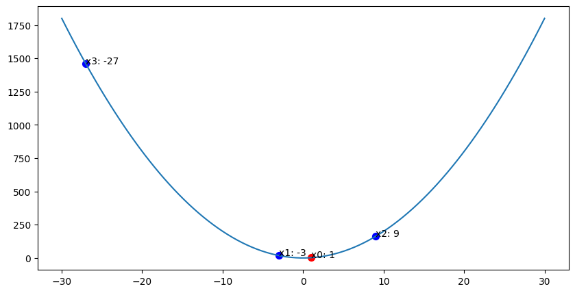
발산 예시
1
2
3
4
5
6
7
8
9
10
11
12
13
14
15
16
17
18
19
20
21
22
23
24
25
26
27
import numpy as np
import matplotlib.pyplot as plt

x_ax = []
y_ax = []
function_x = np.linspace(-30, 30, 100)
function_y = 2*function_x**2

fig, ax = plt.subplots(figsize = (10, 5))
ax.plot(function_x, function_y)
x = 1
y = 2*x**2
ax.scatter(x, y, color = 'red', s= 50 )
x_ax.append(x)
y_ax.append(y)
for _ in range(3):
	dy_dx = 4*x
	x = x - dy_dx
	y = 2*x**2
	ax.scatter(x, y, color = 'blue', s= 50)
	x_ax.append(x)
	y_ax.append(y)

print("x: ", x_ax)
print("y: ", y_ax)
for i, text in enumerate(x_ax):
	ax.annotate(f'x{i}: ' + str(text), (x_ax[i],y_ax[i]))
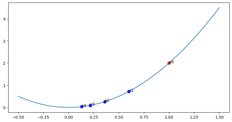
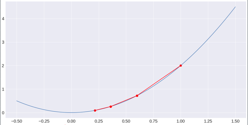
수렴 예시
1
2
3
4
5
6
7
8
9
10
11
12
13
14
15
16
17
18
19
20
21
22
23
24
25
26
27
28
29
30
31
import numpy as np
import matplotlib.pyplot as plt

x_ax = []
y_ax = []

function_x = np.linspace(-0.5, 1.5, 100)
function_y = 2*function_x**2

fig, ax = plt.subplots(figsize = (10, 5))
ax.plot(function_x, function_y)

x = 1
y = 2*x**2
lr = 0.1
ax.scatter(x, y, color = 'red', s= 50)
x_ax.append(x)
y_ax.append(y)

for _ in range(4):
	dy_dx = 4*x
	x = x - lr*dy_dx
	y = 2*x**2
	ax.scatter(x, y, color = 'blue', s= 50)
	x_ax.append(x)
	y_ax.append(y)

print("x: ", x_ax)
print("y: ", y_ax)
for i, text in enumerate(x_ax):
	ax.annotate(f'x{i}', (x_ax[i],y_ax[i]))
Linear Regression with Gradient Descent
1
2
3
4
5
6
7
8
9
10
11
12
13
14
15
16
17
18
19
20
21
22
23
24
25
26
27
28
29
30
31
32
33
34
35
36
37
38
39
40
41
42
43
44
45
46
47
48
49
50
51
52
53
54
55
56
57
58
59
60
61
62
63
64
65
66
67
68
69
70
71
72
73
74
75
76
77
78
79
80
81
82
83
84
85
86
87
88
89
90
91
import numpy as np
import matplotlib.pyplot as plt
# 데이터 생성
X = np.array([1, 2, 3, 4, 5])
y = np.array([2, 4, 5, 4, 5])
# 모델 파라미터 초기화
w = 0
b = 0
# 하이퍼파라미터
learning_rate = 0.01
epochs = 100
# 손실과 파라미터 기록
losses = []
w_history = []
b_history = []
# 경사 하강법
for epoch in range(epochs):
# 예측
y_pred = w * X + b
# 손실 계산 (평균 제곱 오차)
loss = np.mean((y - y_pred) ** 2)
losses.append(loss)
# 그래디언트 계산
dw = -2 * np.mean(X * (y - y_pred))
db = -2 * np.mean(y - y_pred)
# 파라미터 업데이트
w -= learning_rate * dw
b -= learning_rate * db
# 파라미터 기록
w_history.append(w)
b_history.append(b)
if epoch % 10 == 0:
print(f"Epoch {epoch}, Loss: {loss:.4f}, w: {w:.4f}, b: {b:.4f}")
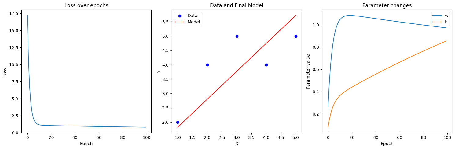
# 결과 시각화
plt.figure(figsize=(15, 5))
# 손실 그래프
plt.subplot(131)
plt.plot(losses)
plt.title('Loss over epochs')
plt.xlabel('Epoch')
plt.ylabel('Loss')
# 데이터와 최종 모델
plt.subplot(132)
plt.scatter(X, y, color='b', label='Data')
plt.plot(X, w * X + b, color='r', label='Model')
plt.title('Data and Final Model')
plt.xlabel('X')
plt.ylabel('y')
plt.legend()
# 파라미터 변화
plt.subplot(133)
plt.plot(w_history, label='w')
plt.plot(b_history, label='b')
plt.title('Parameter changes')
plt.xlabel('Epoch')
plt.ylabel('Parameter value')
plt.legend()
plt.tight_layout()
plt.show()
print(f"Final parameters: w = {w:.4f}, b = {b:.4f}")
'''
Epoch 0, Loss: 17.2000, w: 0.2640, b: 0.0800
Epoch 10, Loss: 1.1595, w: 1.0464, b: 0.3642
Epoch 20, Loss: 1.0475, w: 1.0834, b: 0.4397
Epoch 30, Loss: 1.0100, w: 1.0708, b: 0.4993
Epoch 40, Loss: 0.9753, w: 1.0553, b: 0.5560
Epoch 50, Loss: 0.9429, w: 1.0402, b: 0.6107
Epoch 60, Loss: 0.9125, w: 1.0255, b: 0.6637
Epoch 70, Loss: 0.8842, w: 1.0114, b: 0.7148
Epoch 80, Loss: 0.8577, w: 0.9977, b: 0.7643
Epoch 90, Loss: 0.8330, w: 0.9844, b: 0.8121
Final parameters: w = 0.9729, b = 0.8538
'''